# Installing required python packages
! pip install rich numpy pandas pyarrow matplotlib seaborn scikit-learn hyperopt --quietNIST (part 2): Traditional ML: Gradient boosting
Ralf Gabriels 
![]()
1. Introduction
This is the second part in a three-part tutorial. We recommend you to to start with the first section, where the NIST spectral library is parsed and prepared for use in the second and third parts.
In this tutorial, you will learn how to build a fragmentation intensity predictor similar to MS²PIP v3 (Gabriels, Martens, and Degroeve 2019) with traditional machine learning (ML) feature engineering and Gradient Boosting (Friedman 2002).
2 Data preparation
We will use the spectral library that was already parsed in part 1 of this tutorial series.
import pandas as pd

train_val_spectra = pd.read_feather("http://ftp.pride.ebi.ac.uk/pub/databases/pride/resources/proteomicsml/fragmentation/nist-humanhcd20160503-parsed-trainval.feather")
test_spectra = pd.read_feather("http://ftp.pride.ebi.ac.uk/pub/databases/pride/resources/proteomicsml/fragmentation/nist-humanhcd20160503-parsed-test.feather")
2.1 Feature engineering
In traditional ML, the input features for the algorithm usually require some engineering. For fragmentation intensity prediction this is not different. Following the MS²PIP methods, we will calculate the distributions of several amino acid properties across the peptide and fragment ion sequences.
Using the distribution of these properties instead of the actual properties per amino acid allows MS²PIP to get a fixed length feature matrix for input peptides with varying lengths.
import numpy as np
import pandas as pd
from rich import progress
amino_acids = list("ACDEFGHIKLMNPQRSTVWY")
properties = np.array([
[37,35,59,129,94,0,210,81,191,81,106,101,117,115,343,49,90,60,134,104], # basicity
[68,23,33,29,70,58,41,73,32,73,66,38,0,40,39,44,53,71,51,55], # helicity
[51,75,25,35,100,16,3,94,0,94,82,12,0,22,22,21,39,80,98,70], # hydrophobicity
[32,23,0,4,27,32,48,32,69,32,29,26,35,28,79,29,28,31,31,28], # pI
])
pd.DataFrame(properties, columns=amino_acids, index=["basicity", "helicity", "hydrophobicity", "pI"])| A | C | D | E | F | G | H | I | K | L | M | N | P | Q | R | S | T | V | W | Y | |
|---|---|---|---|---|---|---|---|---|---|---|---|---|---|---|---|---|---|---|---|---|
| basicity | 37 | 35 | 59 | 129 | 94 | 0 | 210 | 81 | 191 | 81 | 106 | 101 | 117 | 115 | 343 | 49 | 90 | 60 | 134 | 104 |
| helicity | 68 | 23 | 33 | 29 | 70 | 58 | 41 | 73 | 32 | 73 | 66 | 38 | 0 | 40 | 39 | 44 | 53 | 71 | 51 | 55 |
| hydrophobicity | 51 | 75 | 25 | 35 | 100 | 16 | 3 | 94 | 0 | 94 | 82 | 12 | 0 | 22 | 22 | 21 | 39 | 80 | 98 | 70 |
| pI | 32 | 23 | 0 | 4 | 27 | 32 | 48 | 32 | 69 | 32 | 29 | 26 | 35 | 28 | 79 | 29 | 28 | 31 | 31 | 28 |
def encode_peptide(sequence, charge):
    # 4 properties * 5 quantiles * 3 ion types + 4 properties * 4 site + 2 global
    n_features = 78
    quantiles = [0, 0.25, 0.5, 0.75, 1]
    n_ions = len(sequence) - 1

    # Encode amino acids as integers to index amino acid properties for peptide sequence
    aa_indices = {aa: i for i, aa in  enumerate("ACDEFGHIKLMNPQRSTVWY")}
    aa_to_index = np.vectorize(lambda aa: aa_indices[aa])
    peptide_indexed = aa_to_index(np.array(list(sequence)))
    peptide_properties = properties[:, peptide_indexed]

    # Empty peptide_features array
    peptide_features = np.full((n_ions, n_features), np.nan)

    for b_ion_number in range(1, n_ions + 1):
        # Calculate quantiles of features across peptide, b-ion, and y-ion
        peptide_quantiles = np.hstack(
            np.quantile(peptide_properties, quantiles, axis=1).transpose()
        )
        b_ion_quantiles = np.hstack(
            np.quantile(peptide_properties[:,:b_ion_number], quantiles, axis=1).transpose()
        )
        y_ion_quantiles = np.hstack(
            np.quantile(peptide_properties[:,b_ion_number:], quantiles, axis=1).transpose()
        )

        # Properties on specific sites: nterm, frag-1, frag+1, cterm
        specific_site_indexes = np.array([0, b_ion_number - 1, b_ion_number, -1])
        specific_site_properties = np.hstack(peptide_properties[:, specific_site_indexes].transpose())

        # Global features: Length and charge
        global_features = np.array([len(sequence), int(charge)])

        # Assign to peptide_features array
        peptide_features[b_ion_number - 1, 0:20] = peptide_quantiles
        peptide_features[b_ion_number - 1, 20:40] = b_ion_quantiles
        peptide_features[b_ion_number - 1, 40:60] = y_ion_quantiles
        peptide_features[b_ion_number - 1, 60:76] = specific_site_properties
        peptide_features[b_ion_number - 1, 76:78] = global_features

    return peptide_features


def generate_feature_names():
    feature_names = []
    for level in ["peptide", "b", "y"]:
        for aa_property in ["basicity", "helicity", "hydrophobicity", "pi"]:
            for quantile in ["min", "q1", "q2", "q3", "max"]:
                feature_names.append("_".join([level, aa_property, quantile]))
    for site in ["nterm", "fragmin1", "fragplus1", "cterm"]:
        for aa_property in ["basicity", "helicity", "hydrophobicity", "pi"]:
            feature_names.append("_".join([site, aa_property]))

    feature_names.extend(["length", "charge"])
    return feature_names
Let’s test it with a single peptide. Feel free to use your own name as a “peptide”; as long as it does not contain any non-amino acid characters.
peptide_features = pd.DataFrame(encode_peptide("RALFGARIELS", 2), columns=generate_feature_names())
peptide_features| peptide_basicity_min | peptide_basicity_q1 | peptide_basicity_q2 | peptide_basicity_q3 | peptide_basicity_max | peptide_helicity_min | peptide_helicity_q1 | peptide_helicity_q2 | peptide_helicity_q3 | peptide_helicity_max | ... | fragplus1_basicity | fragplus1_helicity | fragplus1_hydrophobicity | fragplus1_pi | cterm_basicity | cterm_helicity | cterm_hydrophobicity | cterm_pi | length | charge | |
|---|---|---|---|---|---|---|---|---|---|---|---|---|---|---|---|---|---|---|---|---|---|
| 0 | 0.0 | 43.0 | 81.0 | 111.5 | 343.0 | 29.0 | 41.5 | 68.0 | 71.5 | 73.0 | ... | 37.0 | 68.0 | 51.0 | 32.0 | 49.0 | 44.0 | 21.0 | 29.0 | 11.0 | 2.0 |
| 1 | 0.0 | 43.0 | 81.0 | 111.5 | 343.0 | 29.0 | 41.5 | 68.0 | 71.5 | 73.0 | ... | 81.0 | 73.0 | 94.0 | 32.0 | 49.0 | 44.0 | 21.0 | 29.0 | 11.0 | 2.0 |
| 2 | 0.0 | 43.0 | 81.0 | 111.5 | 343.0 | 29.0 | 41.5 | 68.0 | 71.5 | 73.0 | ... | 94.0 | 70.0 | 100.0 | 27.0 | 49.0 | 44.0 | 21.0 | 29.0 | 11.0 | 2.0 |
| 3 | 0.0 | 43.0 | 81.0 | 111.5 | 343.0 | 29.0 | 41.5 | 68.0 | 71.5 | 73.0 | ... | 0.0 | 58.0 | 16.0 | 32.0 | 49.0 | 44.0 | 21.0 | 29.0 | 11.0 | 2.0 |
| 4 | 0.0 | 43.0 | 81.0 | 111.5 | 343.0 | 29.0 | 41.5 | 68.0 | 71.5 | 73.0 | ... | 37.0 | 68.0 | 51.0 | 32.0 | 49.0 | 44.0 | 21.0 | 29.0 | 11.0 | 2.0 |
| 5 | 0.0 | 43.0 | 81.0 | 111.5 | 343.0 | 29.0 | 41.5 | 68.0 | 71.5 | 73.0 | ... | 343.0 | 39.0 | 22.0 | 79.0 | 49.0 | 44.0 | 21.0 | 29.0 | 11.0 | 2.0 |
| 6 | 0.0 | 43.0 | 81.0 | 111.5 | 343.0 | 29.0 | 41.5 | 68.0 | 71.5 | 73.0 | ... | 81.0 | 73.0 | 94.0 | 32.0 | 49.0 | 44.0 | 21.0 | 29.0 | 11.0 | 2.0 |
| 7 | 0.0 | 43.0 | 81.0 | 111.5 | 343.0 | 29.0 | 41.5 | 68.0 | 71.5 | 73.0 | ... | 129.0 | 29.0 | 35.0 | 4.0 | 49.0 | 44.0 | 21.0 | 29.0 | 11.0 | 2.0 |
| 8 | 0.0 | 43.0 | 81.0 | 111.5 | 343.0 | 29.0 | 41.5 | 68.0 | 71.5 | 73.0 | ... | 81.0 | 73.0 | 94.0 | 32.0 | 49.0 | 44.0 | 21.0 | 29.0 | 11.0 | 2.0 |
| 9 | 0.0 | 43.0 | 81.0 | 111.5 | 343.0 | 29.0 | 41.5 | 68.0 | 71.5 | 73.0 | ... | 49.0 | 44.0 | 21.0 | 29.0 | 49.0 | 44.0 | 21.0 | 29.0 | 11.0 | 2.0 |
10 rows × 78 columns
2.2 Getting the target intensities
The target intensities are the observed intensities which the model will learn to predict. Let’s first try with a single spectrum.
test_spectrum = train_val_spectra.iloc[4]

peptide_targets =  pd.DataFrame({
    "b_target": test_spectrum["parsed_intensity"]["b"],
    "y_target": test_spectrum["parsed_intensity"]["y"],
})
peptide_targets| b_target | y_target | |
|---|---|---|
| 0 | 0.000000 | 0.118507 |
| 1 | 0.229717 | 0.079770 |
| 2 | 0.294631 | 0.088712 |
| 3 | 0.234662 | 0.145900 |
| 4 | 0.185732 | 0.205005 |
| 5 | 0.134395 | 0.261630 |
| 6 | 0.081856 | 0.305119 |
| 7 | 0.043793 | 0.296351 |
| 8 | 0.000000 | 0.205703 |
| 9 | 0.000000 | 0.155991 |
| 10 | 0.000000 | 0.000000 |
These are the intensities for the b- and y-ions, each ordered from 1 to 9. In MS²PIP, however, a clever trick is applied to reuse the computed features for each fragment ion pair. Doing so makes perfect sense, as both ions in such a fragment ion pair originated from the same fragmentation event. For this peptide, the fragment ion pairs are b1-y9, b2-y8, b3-y7, etc. To match all of the pairs, we simply have to reverse the y-ion series intensities:
peptide_targets =  pd.DataFrame({
    "b_target": test_spectrum["parsed_intensity"]["b"],
    "y_target": test_spectrum["parsed_intensity"]["y"][::-1],
})
peptide_targets| b_target | y_target | |
|---|---|---|
| 0 | 0.000000 | 0.000000 |
| 1 | 0.229717 | 0.155991 |
| 2 | 0.294631 | 0.205703 |
| 3 | 0.234662 | 0.296351 |
| 4 | 0.185732 | 0.305119 |
| 5 | 0.134395 | 0.261630 |
| 6 | 0.081856 | 0.205005 |
| 7 | 0.043793 | 0.145900 |
| 8 | 0.000000 | 0.088712 |
| 9 | 0.000000 | 0.079770 |
| 10 | 0.000000 | 0.118507 |
2.3 Bringing it all together
features = encode_peptide(test_spectrum["sequence"], test_spectrum["charge"])
targets = np.stack([test_spectrum["parsed_intensity"]["b"], test_spectrum["parsed_intensity"]["y"][::-1]], axis=1)
spectrum_id = np.full(shape=(targets.shape[0], 1), fill_value=test_spectrum["index"])  # Repeat id for all ions
pd.DataFrame(np.hstack([spectrum_id, features, targets]), columns=["spectrum_id"] + generate_feature_names() + ["b_target", "y_target"])| spectrum_id | peptide_basicity_min | peptide_basicity_q1 | peptide_basicity_q2 | peptide_basicity_q3 | peptide_basicity_max | peptide_helicity_min | peptide_helicity_q1 | peptide_helicity_q2 | peptide_helicity_q3 | ... | fragplus1_hydrophobicity | fragplus1_pi | cterm_basicity | cterm_helicity | cterm_hydrophobicity | cterm_pi | length | charge | b_target | y_target | |
|---|---|---|---|---|---|---|---|---|---|---|---|---|---|---|---|---|---|---|---|---|---|
| 0 | 5.0 | 37.0 | 37.0 | 37.0 | 40.0 | 343.0 | 39.0 | 68.0 | 68.0 | 68.0 | ... | 51.0 | 32.0 | 343.0 | 39.0 | 22.0 | 79.0 | 12.0 | 2.0 | 0.000000 | 0.000000 |
| 1 | 5.0 | 37.0 | 37.0 | 37.0 | 40.0 | 343.0 | 39.0 | 68.0 | 68.0 | 68.0 | ... | 51.0 | 32.0 | 343.0 | 39.0 | 22.0 | 79.0 | 12.0 | 2.0 | 0.229717 | 0.155991 |
| 2 | 5.0 | 37.0 | 37.0 | 37.0 | 40.0 | 343.0 | 39.0 | 68.0 | 68.0 | 68.0 | ... | 51.0 | 32.0 | 343.0 | 39.0 | 22.0 | 79.0 | 12.0 | 2.0 | 0.294631 | 0.205703 |
| 3 | 5.0 | 37.0 | 37.0 | 37.0 | 40.0 | 343.0 | 39.0 | 68.0 | 68.0 | 68.0 | ... | 51.0 | 32.0 | 343.0 | 39.0 | 22.0 | 79.0 | 12.0 | 2.0 | 0.234662 | 0.296351 |
| 4 | 5.0 | 37.0 | 37.0 | 37.0 | 40.0 | 343.0 | 39.0 | 68.0 | 68.0 | 68.0 | ... | 51.0 | 32.0 | 343.0 | 39.0 | 22.0 | 79.0 | 12.0 | 2.0 | 0.185732 | 0.305119 |
| 5 | 5.0 | 37.0 | 37.0 | 37.0 | 40.0 | 343.0 | 39.0 | 68.0 | 68.0 | 68.0 | ... | 51.0 | 32.0 | 343.0 | 39.0 | 22.0 | 79.0 | 12.0 | 2.0 | 0.134395 | 0.261630 |
| 6 | 5.0 | 37.0 | 37.0 | 37.0 | 40.0 | 343.0 | 39.0 | 68.0 | 68.0 | 68.0 | ... | 51.0 | 32.0 | 343.0 | 39.0 | 22.0 | 79.0 | 12.0 | 2.0 | 0.081856 | 0.205005 |
| 7 | 5.0 | 37.0 | 37.0 | 37.0 | 40.0 | 343.0 | 39.0 | 68.0 | 68.0 | 68.0 | ... | 51.0 | 32.0 | 343.0 | 39.0 | 22.0 | 79.0 | 12.0 | 2.0 | 0.043793 | 0.145900 |
| 8 | 5.0 | 37.0 | 37.0 | 37.0 | 40.0 | 343.0 | 39.0 | 68.0 | 68.0 | 68.0 | ... | 80.0 | 31.0 | 343.0 | 39.0 | 22.0 | 79.0 | 12.0 | 2.0 | 0.000000 | 0.088712 |
| 9 | 5.0 | 37.0 | 37.0 | 37.0 | 40.0 | 343.0 | 39.0 | 68.0 | 68.0 | 68.0 | ... | 21.0 | 29.0 | 343.0 | 39.0 | 22.0 | 79.0 | 12.0 | 2.0 | 0.000000 | 0.079770 |
| 10 | 5.0 | 37.0 | 37.0 | 37.0 | 40.0 | 343.0 | 39.0 | 68.0 | 68.0 | 68.0 | ... | 22.0 | 79.0 | 343.0 | 39.0 | 22.0 | 79.0 | 12.0 | 2.0 | 0.000000 | 0.118507 |
11 rows × 81 columns
The following function applies these steps over a collection of spectra and returns the full feature/target table:
def generate_ml_input(spectra):
    tables = []
    for spectrum in progress.track(spectra.to_dict(orient="records")):
        features = encode_peptide(spectrum["sequence"], spectrum["charge"])
        targets = np.stack([spectrum["parsed_intensity"]["b"], spectrum["parsed_intensity"]["y"][::-1]], axis=1)
        spectrum_id = np.full(shape=(targets.shape[0], 1), fill_value=spectrum["index"])  # Repeat id for all ions
        table = np.hstack([spectrum_id, features, targets])
        tables.append(table)

    full_table = np.vstack(tables)
    spectra_encoded = pd.DataFrame(full_table, columns=["spectrum_id"] + generate_feature_names() + ["b_target",  "y_target"])
    return spectra_encoded
Note that this might take some time, sometimes up to 30 minutes. To skip this step, simple download the file with pre-encoded features and targets, and load in two cells below.
train_val_encoded = generate_ml_input(train_val_spectra)
train_val_encoded.to_feather("fragmentation-nist-humanhcd20160503-parsed-trainval-encoded.feather")

test_encoded = generate_ml_input(test_spectra)
test_encoded.to_feather("fragmentation-nist-humanhcd20160503-parsed-test-encoded.feather")
# Uncomment this step to load pre-encoded features from a file:
# train_val_encoded = pd.read_feather("http://ftp.pride.ebi.ac.uk/pub/databases/pride/resources/proteomicsml/fragmentation/nist-humanhcd20160503-parsed-trainval-encoded.feather")
# test_encoded = pd.read_feather("http://ftp.pride.ebi.ac.uk/pub/databases/pride/resources/proteomicsml/fragmentation/nist-humanhcd20160503-parsed-test-encoded.feather")train_val_encoded| spectrum_id | peptide_basicity_min | peptide_basicity_q1 | peptide_basicity_q2 | peptide_basicity_q3 | peptide_basicity_max | peptide_helicity_min | peptide_helicity_q1 | peptide_helicity_q2 | peptide_helicity_q3 | ... | fragplus1_hydrophobicity | fragplus1_pi | cterm_basicity | cterm_helicity | cterm_hydrophobicity | cterm_pi | length | charge | b_target | y_target | |
|---|---|---|---|---|---|---|---|---|---|---|---|---|---|---|---|---|---|---|---|---|---|
| 0 | 0.0 | 0.0 | 37.0 | 37.0 | 37.0 | 191.0 | 32.0 | 68.0 | 68.0 | 68.0 | ... | 51.0 | 32.0 | 191.0 | 32.0 | 0.0 | 69.0 | 22.0 | 2.0 | 0.000000 | 0.000000 |
| 1 | 0.0 | 0.0 | 37.0 | 37.0 | 37.0 | 191.0 | 32.0 | 68.0 | 68.0 | 68.0 | ... | 51.0 | 32.0 | 191.0 | 32.0 | 0.0 | 69.0 | 22.0 | 2.0 | 0.094060 | 0.000000 |
| 2 | 0.0 | 0.0 | 37.0 | 37.0 | 37.0 | 191.0 | 32.0 | 68.0 | 68.0 | 68.0 | ... | 51.0 | 32.0 | 191.0 | 32.0 | 0.0 | 69.0 | 22.0 | 2.0 | 0.180642 | 0.000000 |
| 3 | 0.0 | 0.0 | 37.0 | 37.0 | 37.0 | 191.0 | 32.0 | 68.0 | 68.0 | 68.0 | ... | 51.0 | 32.0 | 191.0 | 32.0 | 0.0 | 69.0 | 22.0 | 2.0 | 0.204203 | 0.050476 |
| 4 | 0.0 | 0.0 | 37.0 | 37.0 | 37.0 | 191.0 | 32.0 | 68.0 | 68.0 | 68.0 | ... | 51.0 | 32.0 | 191.0 | 32.0 | 0.0 | 69.0 | 22.0 | 2.0 | 0.233472 | 0.094835 |
| ... | ... | ... | ... | ... | ... | ... | ... | ... | ... | ... | ... | ... | ... | ... | ... | ... | ... | ... | ... | ... | ... |
| 3321136 | 398372.0 | 81.0 | 104.0 | 104.0 | 153.0 | 343.0 | 39.0 | 48.5 | 55.0 | 55.0 | ... | 70.0 | 28.0 | 343.0 | 39.0 | 22.0 | 79.0 | 8.0 | 3.0 | 0.000000 | 0.180938 |
| 3321137 | 398372.0 | 81.0 | 104.0 | 104.0 | 153.0 | 343.0 | 39.0 | 48.5 | 55.0 | 55.0 | ... | 98.0 | 31.0 | 343.0 | 39.0 | 22.0 | 79.0 | 8.0 | 3.0 | 0.000000 | 0.203977 |
| 3321138 | 398372.0 | 81.0 | 104.0 | 104.0 | 153.0 | 343.0 | 39.0 | 48.5 | 55.0 | 55.0 | ... | 3.0 | 48.0 | 343.0 | 39.0 | 22.0 | 79.0 | 8.0 | 3.0 | 0.000000 | 0.169803 |
| 3321139 | 398372.0 | 81.0 | 104.0 | 104.0 | 153.0 | 343.0 | 39.0 | 48.5 | 55.0 | 55.0 | ... | 94.0 | 32.0 | 343.0 | 39.0 | 22.0 | 79.0 | 8.0 | 3.0 | 0.000000 | 0.120565 |
| 3321140 | 398372.0 | 81.0 | 104.0 | 104.0 | 153.0 | 343.0 | 39.0 | 48.5 | 55.0 | 55.0 | ... | 22.0 | 79.0 | 343.0 | 39.0 | 22.0 | 79.0 | 8.0 | 3.0 | 0.000000 | 0.169962 |
3321141 rows × 81 columns
This is the data we will use for training. Note that each spectrum comprises of multiple lines: One line per b/y-ion couple.
3 Training the model
from sklearn.ensemble import GradientBoostingRegressorLet’s first try to train a simple model on the train set and evaluate its performance on the test set.
reg =  GradientBoostingRegressor()

X_train = train_val_encoded.drop(columns=["spectrum_id", "b_target",  "y_target"])
y_train = train_val_encoded["y_target"]
X_test = test_encoded.drop(columns=["spectrum_id", "b_target",  "y_target"])
y_test = test_encoded["y_target"]

# For demo purposes, we only use the first 100k samples
reg.fit(X_train.head(100000), y_train.head(100000))

# Uncomment this step to train the model on the full dataset:
# reg.fit(X_train, y_train)GradientBoostingRegressor()In a Jupyter environment, please rerun this cell to show the HTML representation or trust the notebook.
On GitHub, the HTML representation is unable to render, please try loading this page with nbviewer.org.
GradientBoostingRegressor()
y_test_pred = reg.predict(X_test)
np.corrcoef(y_test, y_test_pred)[0][1]0.7091798896983967Not terrible. Let’s see if we can do better after hyperparameters optimization. For this, we can use the hyperopt package.
from hyperopt import fmin, hp, tpe, STATUS_OKdef objective(n_estimators):
# Define algorithm
reg = GradientBoostingRegressor(n_estimators=n_estimators)
# Fit model
# For demo purposes, we only use the first 100k samples
reg.fit(X_train.head(100000), y_train.head(100000))
# Uncomment this step to train the model on the full dataset:
# reg.fit(X_train, y_train)
# Test model
y_test_pred = reg.predict(X_test)
correlation = np.corrcoef(y_test, y_test_pred)[0][1]
return {'loss': -correlation, 'status': STATUS_OK}best_params = fmin(
fn=objective,
space=10 + hp.randint('n_estimators', 980),
algo=tpe.suggest,
max_evals=10,
)100%|██████████| 10/10 [37:15<00:00, 223.58s/trial, best loss: -0.75991576993057] best_params{'n_estimators': 966}Initially, the default value of 100 estimators was used. According to this hyperopt run, using 966 estimators results in a more performant model.
Now we can train the model again with this new hyperparameter value:
reg =  GradientBoostingRegressor(n_estimators=best_params["n_estimators"])

X_train = train_val_encoded.drop(columns=["spectrum_id", "b_target",  "y_target"])
y_train = train_val_encoded["y_target"]
X_test = test_encoded.drop(columns=["spectrum_id", "b_target",  "y_target"])
y_test = test_encoded["y_target"]

reg.fit(X_train.head(100000), y_train.head(100000))GradientBoostingRegressor(n_estimators=966)In a Jupyter environment, please rerun this cell to show the HTML representation or trust the notebook.
On GitHub, the HTML representation is unable to render, please try loading this page with nbviewer.org.
GradientBoostingRegressor(n_estimators=966)
y_test_pred = reg.predict(X_test)
np.corrcoef(y_test, y_test_pred)[0][1]0.7593069387129985Much better already. To get a more accurate view of the model performance, we should calculate the correlation per spectrum, instead of across the full dataset:
prediction_df_y = pd.DataFrame({
    "spectrum_id": test_encoded["spectrum_id"],
    "target_y": y_test,
    "prediction_y": y_test_pred,
})
prediction_df_y| spectrum_id | target_y | prediction_y | |
|---|---|---|---|
| 0 | 9.0 | 0.000000 | 0.006154 |
| 1 | 9.0 | 0.000000 | 0.008823 |
| 2 | 9.0 | 0.000000 | 0.010059 |
| 3 | 9.0 | 0.000000 | 0.011024 |
| 4 | 9.0 | 0.000000 | 0.019898 |
| ... | ... | ... | ... |
| 367683 | 398369.0 | 0.000000 | 0.262313 |
| 367684 | 398369.0 | 0.224074 | 0.268292 |
| 367685 | 398369.0 | 0.283664 | 0.208505 |
| 367686 | 398369.0 | 0.185094 | 0.177186 |
| 367687 | 398369.0 | 0.192657 | 0.263046 |
367688 rows × 3 columns
corr_y = prediction_df_y.groupby("spectrum_id").corr().iloc[::2]['prediction_y']
corr_y.index = corr_y.index.droplevel(1)
corr_y = corr_y.reset_index().rename(columns={"prediction_y": "correlation"})
corr_y| spectrum_id | correlation | |
|---|---|---|
| 0 | 9.0 | 0.868330 |
| 1 | 16.0 | 0.725240 |
| 2 | 39.0 | 0.101923 |
| 3 | 95.0 | 0.118734 |
| 4 | 140.0 | 0.785892 |
| ... | ... | ... |
| 27031 | 398328.0 | 0.675631 |
| 27032 | 398341.0 | 0.066689 |
| 27033 | 398342.0 | 0.763430 |
| 27034 | 398368.0 | 0.684804 |
| 27035 | 398369.0 | -0.352181 |
27036 rows × 2 columns
Median correlation:
corr_y["correlation"].median()0.7524246447174651Correlation distribution:
import matplotlib.pyplot as plt
import seaborn as sns
sns.set_style("whitegrid")
sns.catplot(
data=corr_y, x="correlation",
fliersize=1,
kind="box", aspect=4, height=2
)
plt.show()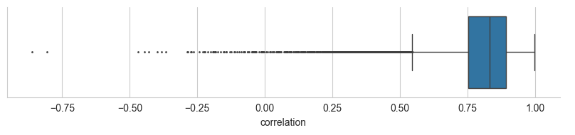
Not bad! With some more hyperparameter optimization (optimizing only the number of trees is a bit crude) a lot more performance gains could be made. Take a look at the Scikit Learn documentation to learn more about the various hyperparameters for the GradientBoostingRegressor. Alternatively, you could switch to the XGBoost algorithm, which is currently used by MS²PIP.
And of course, this model can only predict y-ion intensities. You can repeat the training and optimization steps to train a model for b-ion intensities.
Good luck!
References
Friedman, Jerome H. 2002. “Stochastic Gradient Boosting.” Computational Statistics and Data Analysis 38 (4): 367–78. https://doi.org/10.1016/s0167-9473(01)00065-2.
Gabriels, Ralf, Lennart Martens, and Sven Degroeve. 2019. “Updated MS²PIP Web Server Delivers Fast and Accurate MS² Peak Intensity Prediction for Multiple Fragmentation Methods, Instruments and Labeling Techniques.” NUCLEIC ACIDS RESEARCH 47 (W1): W295–99. https://doi.org/10.1093/nar/gkz299.